


Diagnostic studies: some biometric basics
What is diagnostics anyway?
No answer should be given here, because one would have to start with philosophical discussions of the cognitive process ... and continue with the principles of medical action. The terms illness, diagnosis, diagnostics, test, diagnostic process etc. should be defined. - The biometrician can make things easy for him: he sees the diagnostic measure as a means, an a priori probability for the correctness of the presumption that a patient suffers from an illness, in a (possible) higher a posteriori probability transform.
From diagnostics to diagnostic tests
In order to describe the diagnosis, it is interpreted as a sequence of binary individual decisions. These individual distinctions use diagnostic tests that are supposed to decide between two conditions: disease present / not present. Accordingly, the test result is a yes / no statement: sick (= positive) / not sick (= negative). For tests with quantitative results, such as B. for laboratory values, the conversion into such a binary statement takes place with a cut-off value (Cut-off point).
From this, a four-field table can be created that compares the patient's true condition (reference standard, gold standard) and the test result (examined test = index test):
| Reference standard: Disease D | Reference standard: non-disease D- | |
|---|---|---|
| Index test: test positive T | True positive test result: TP | False positive test result: FP |
| Index test: test negative T- | False negative test result: FN | True negative test result: TN |
Diagnostic quality measures
On this table, the ratios of the individual cells to the sums can be formed in columns and rows.
First we can give the prevalence: D + / ([D +] + [D-]) = (TP + TN) / (TP + FP + TN + FN).
Diagnostic quality is always reported as a pair of two values: {sensitivity, specificity}, or {PPV, NPV} or {DLR +, DLR-}.
Summary measures that only use one value (e.g. sum of sensitivity and specificity, Youden index, efficiency, ...) do not and do not adequately reflect the quality of a test not suitableto describe the diagnostic goodness. If only a number is reported (eg only the negative predictive value, or an "accuracy of 95%", etc., this information is not sufficient to assess the quality of a diagnostic test. I personally go in such cases assume that an unfavorable property of the test should be kept secret.
The sensitivity determines the proportion of the patients who are correctly recognized as positive in all patients TP / D + = TP / (TP + FN), the specificity the proportion of the patients who are recognized as really negative in the non-patients TN / D- = TN / (TN + FP ). The grades can also be formulated statistically as conditional probabilities: the sensitivity is the conditional probability of having a really positive test result given the disease [this is noted: P (T + | D +)], the specificity is the conditional probability of being present given a really negative test result, the non-disease P (T- | D-). Sensitivity and specificity are the quantities that developers and manufacturers can use when evaluating their diagnostic tests. Instead of sensitivity, the correct-positive rate TPF = sensitivity and false-positive rate = 1-specificity are also sometimes given. Since sensitivity and specificity are determined within the columns of the table reported above, they do not depend on the prevalence.
The predictive values (line-by-line consideration), on the other hand, consider the probabilities that the patient actually has the condition that the test indicates (positive predictive value PPV: TP / (TP + FP), negative predictive value NPV: TN / (TN + FN) also formulate the predictive values statistically as conditional probabilities: the PPV is the conditional probability of a disease being given a positive test result P (D + | T +) [note the reversed order of T + and D + compared to sensitivity], the NPV is that conditional probability for the existence of a non-disease given a negative test result P (D- | D-). The predicted values thus describe the view of the doctor (or the patient) to whom the test result is available: I have a positive test result: how high is it Probability that I am actually ill? The PPV answers this.Physician and patient can test the test result with the PPV or the NPV assess its relevance.
How can assess whether predictive values are good? This should be explained using the example of the Pap test, a screening test for the presence of cervical lesion (prevalence = 0.8%). The sensitivity is 55%, the specificity 97%. You can then calculate that the Pap test has an (apparently small) positive predictive value of 12.8%, but it is still a good test. This assessment is achieved by comparing the PPV (12.8%) with the prevalence (0.8%) and the NPV (which is 99.6%) with 1 prevalence (99.2%). In this respect, the Pap test offers a clear information gain in the event of a positive test result, since the PPV is significantly larger than the prevalence (12.8% vs. 0.8%).
The positive diagnostic likelihood ratio (DLR +), which together with the negative DLR- can also be used as a measure of the diagnostic quality, forms this information gaindirectly
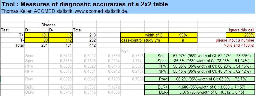
from. The ratio of post-test odds / pretest odds is used. In practice, DLR + is calculated from Sens / (1-Spec) [negative DLR: (1-Sens) / Spez]. The Pap test has a DLR + of 18.3 and a DLR- of 0.46. The diagnostic likelihood ratio is therefore the measure of the diagnostic quality that best reflects the information gained through the test. They are also the only measure whose absolute numbers can be assessed directly. So there is a rough rule of thumb that a test is "good" if DLR +> 3 and DLR- <0.33. Not too many IvD tests achieve this, the tumor marker Cyfra 21-1 is one example, the figure below left.
The following picture shows the calculation of the dimensions of the diagnostic quality using the example of the tumor marker Cyfra 21-1 (data from Keller et al, 1998) as well as an overview table of characteristics of the dimensions of the diagnostic quality (cited from Pepe 2003).


Aims of a diagnostic study
As a rule, the aim of a diagnostic study is to determine the diagnostic quality (together with the confidence interval), whereby the usual measures are the value pairs sensitivity / specificity and / or positive / negative predictive value (abbr .: PPV / NPV). Positive and negative diagnostic likelihood ratio (abbr: DLR + / DLR-) are sometimes requested separately by the authorities or reviewers.
One has to be aware that the study approach of determining (statisticians say: estimate) the diagnostic quality is explorative. A confirmatory approach would consist in the prospectively planned proof that the diagnostic quality exceeds certain values (e.g. proof that Sens> 60%, Spec> 80%). In practice, it is also often the case that there is evidence that the sensitivity exceeds a certain value, while the specificity does not fall below a certain value (non-inferiority).
Another goal is the comparison of diagnostic grades of different diagnostics. Strictly speaking, two comparisons are to be formulated here, each for sensitivity and specificity. Here, too, one often encounters the situation that only one of the measures should be better than that for the comparison test, while for the other measure only non-inferiority has to be shown. RTPF (ratio of sensitivities) and rFPF (ratio of false positive rates [= 1 specificity]) or rPPV (ratio of PPV) and rNPV (ratio of NPV) can be used as comparative studies, since these are statistical models are easily accessible (you can estimate them directly with generalized linear models with logarithm as a link function, including the confidence interval and, if necessary, consideration of influencing factors).
Phases of diagnostic studies
What should you do if you want to examine and evaluate a diagnostic test? Köberberling et al. (1989) distinguish 4 phases, which are still very practical:
Phase I:
The method is examined in a technical preliminary examination. This validation of the measurement properties, e.g. B. Accuracy and precision, provides information on the quality of the method. Further information on Method validation see the section
laboratory
.
Phase II:
Examination of the measured values for distribution differences between different patient groups. This makes it possible to make a statement about the potential of the test. Phase II studies include patients for whom the diagnosis is already established. The number of cases per group is not based on the prevalence of the disease, but on statistical considerations.
Example: For a phase II study on the diagnostic potential of a tumor marker, 150 patients with a histologically proven tumor and 100 patients with an inflammatory disease on the organ in question (tumor exclusion has already occurred) are included. (In this case, it is important to take the blood before starting therapy, since therapy influences the tumor marker content.) - With this procedure, the spectrum of the future application population is not shown correctly, but "sickly" patients and "healthier" non-sick people are preferred.
This spectrum distortion leads to an overestimation of the diagnostic quality. In my experience, this is the main reason for the failure of many biomarkers that initially appear promising: the diagnostic quality was determined in a case-control study.
This can be counteracted to a certain extent by specifically considering various disease stages, various concomitant diseases and various demographic factors when selecting patients.

A phase II study allows statements to be made on the relationship between sensitivity and specificity of the test using an ROC curve (ROC: receiver operating characteristics), whereby, as described, an overestimation can be assumed.
To create the ROC curve, the cut-off point is varied over the range of values of the diagnostic test. The ratios regarding the numbers TP, FP, FN and TN change accordingly. In practice, you use every measured value in the studies and calculate sensitivity and specificity. The result is a curve as in the adjacent figure.
The ROC curve is used for scientific exploration of the diagnostic quality of the test. You can use it for Determination of the cut-off
draw in. The area under the curve (AUC) is an overview measure for the diagnostic quality, but in contrast to the value pairs described above, it is unsuitable for specifying the diagnostic quality of a test.
Illustration:
ROC (receiver operating characteristics) curve, with indication of the confidence band and individual cut-off values. Created with the ACOMED Excel tool, see web shop. Underlying values: CYFRA 21-1 for the diagnosis of bronchial CA in patients with suspected disease [Keller et al. 1998].
ROC (receiver operating characteristics) curve, with indication of the confidence band and individual cut-off values. Created with the ACOMED Excel tool, see web shop. Underlying values: CYFRA 21-1 for the diagnosis of bronchial CA in patients with suspected disease [Keller et al. 1998].
The example above leads to
Phase III study: In a controlled diagnostic study, the test is assessed in the specific clinical application situation.
In a phase III diagnostic study, all patients with a suspected disease are included in the study; the disease status is not yet known. This corresponds exactly to the situation in which the test would be used in the diagnostic routine. The diagnostic procedure for the detection of the disease or its exclusion must be precisely defined and recognized (reference method, gold standard, diagnostic accuracy criterion).
Example: To evaluate a heart attack marker in general practitioners, all patients who have a certain complaint (e.g. breathing difficulties, unclear complaints in the chest area, characteristic disorders of the ECG) must be included in the study. It can be expected that a test that is successfully used in cardiac centers, for example, will have a completely different performance when used in private practice because the patient population is completely different and the prevalence of the target disease differs.
In phase III studies, cut-off values can be set, which is more difficult than commonly assumed. Since there is always an overlap zone ("gray zone"), in which the test gives the same results for the sick and not the sick, it is important to consider: Are false positives or false negatives classified as favorable? Further Notes on determining cut-off values.
Phase IV studies
examine the therapeutic benefit of a therapeutic measure following the diagnostic test (efficacy studies) and answer questions such as these:
- Will the introduction of a new imaging method that can identify smaller tumor areas lead to an increase in survival time?
- Let us consider patients who experience side effects for certain medications. Does a diagnostic test that identifies these patients reduce the complication rate?
Phase IV studies are complex and time-consuming to carry out, and no further description is required here.
Bias in diagnostic studies
Finally, notes on three systematic errors that can occur in addition to other errors in the evaluation of diagnostic tests and lead to biases.
Selection bias / spectrum bias:
This is the main bias in clinical diagnostic studies. The bias is present if the selection of the examined patients or the spectrum of the patients included in the study does not correspond to the clinical application situation. This has already been discussed above in connection with phase II diagnostic studies.
Verification bias:
A significant bias is expected if the reference standard cannot be obtained in the same quality for all patients. For example, an invasive procedure is only used for test positives, while understandably no test negatives are used. An overestimation of the sensitivity can be expected.
Missing blinding, information bias:
Knowledge of the test result of the test to be examined influences the result of the external criterion. This is particularly to be expected for procedures in which findings have to be interpreted (imaging procedures). A particularly common error with regard to removing the blinding is the re-testing (i.e. repeated measurements or extensive testing) of discordant (i.e. false positive or false negative) cases. This is only permissible if a randomly selected sub-sample of concordant cases is also subjected to this procedure. In a FDA guideline (2007)
this aspect is considered in detail for diagnostic studies.
literature
As literature, I particularly recommend the book by MS Pepe. Concerning. the phases of diagnostic studies are the two publications by Köbberling et al. recommended.
Pepe MS (2003): The Statistical Evaluation of Medical Tests for Classification and Prediction. Oxford University Press 2003
Zhou XH, Obuchowski NA, McClish DK (2011, 2nd ed). Statistical Methods in Diagnostic Medicine. Wiley Interscience New York.
Köbberling J, Richter K, Trampisch HJ, Windeler J: Methodology of medical diagnostics. Development, assessment and application of diagnostic procedures in medicine. Springer-Verlag Berlin Heidelberg New-York (1991)
Köbberling J, Trampisch HJ, Windeler J: Memorandum for the evaluation of diagnostic measures. Series of the GMDS (1989) 10
Begg CB: Biases in the Assessment of Diagnostic Tests. Stat. Med. (1987) 6, 411-423
Linnet K: A Review on the Methodology for Assessing Diagnostic Tests. Clin. Chem. (1988) 34, 1379-1386